Introduction
Target Stock Levels (TSL) specifies the optimal equipment stock, required to ensure equipment availability for the local export demand and bookings. TSL is calculated automatically, partly based on the Auto Forecast, and partly based on input from the equipment planners. The auto forecast is used as the main driver for setting TSL because it covers all sites globally and is released automatically every week. The auto forecast is calculated and managed as a weekly import/export total, which means the target stock levels are also managed per week.per week and Furthermore, because the auto forecast data is calculated and managed per week, so is the target stock levels. This page describes the main concepts used to manage the calculate and manage the target stock levels.
Main Concepts
This section describes a few of the main concepts used to calculate and manage TSL.
The Target Stock Level Range
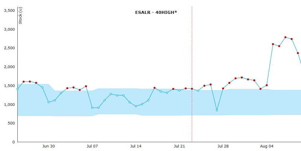
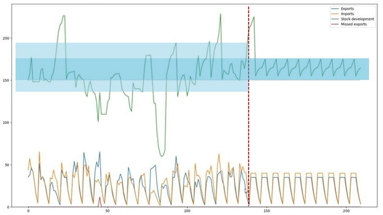
The equipment stock in the depots and terminals are constantly impacted by export pick-ups, import returns, empty re-positioning, and transshipments. Because the timing of these events are independent of each other, the stock level will be very volatile if analysed over a few days. To fairly judge how well the stock is managed it is necessary assess it over time. To support this analysis the optimal stock level is defined as range consisting of a lower bound "TSL MIN" and upper bound "TSL MAX" (see figure A).
TSL MIN specifies the optimal stock level required to ensure a healthy stock level, including relevant buffers, such as equipment preparation. Equipment planning should be done in a way, where stock is balanced around TSL MIN, reaching this level as frequently as possible. If it is not possible to reach TSL MIN frequently, either the target is too low or the depot/terminal has too much surplus stock.
TSL MAX specifies the highest stock level that TSL should ideally reach during the week, considering the balance of trade and positioning options available. TSL only represents the range to satisfy the immediate exports. Going above the TSL max is a natural consequence of building stock for seasonal peaks (dictated by REP).
|
| Figure A: stock performance graph in ROCK for ESALR/40HIGH* |
Forecast Predictions
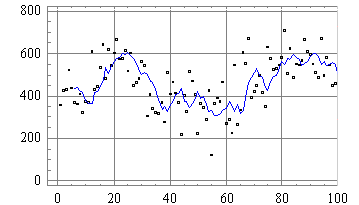
Time-series forecasting (i.e. like the auto forecast in ROCK) takes a history of data points and combines it with a forecasting model that predicts what the future value will be (i.e. the prediction). Furthermore, the spread of the data is captured as the standard deviation (SD) and describes the average spread of population against the mean (see figure B).
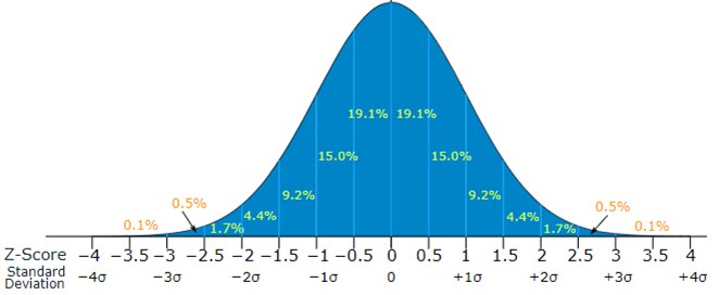
In probability theory, the central limit theorem establishes that, regardless of the population distribution model, as the sample data size increases, the sample mean tends to be normally distributed around the population mean, and its SD shrinks as n increases. This is valid when the samples are independent and the size of the population is large enough. Figure C illustrates this point, where a normally distributed data set will be dispersed around the mean, as a bell-shaped curve, where the standard deviation can be used to capture a subset of the population.
|
|
Figure B: scatter plot of data with trend line | Figure C: bell curve of a standard normal distribution |

Factor applied to the SD (σ) | 0,5σ | 1σ | 1,5σ | 2σ | 2,5σ | 3σ |
Expected fraction of population inside range | 38,2% | 68,2% | 86,6% | 95,4% | 98,7% | 99,7% |
Approximate frequency of events outside of range | 2 in 3 | 1 in 3 | 1 in 7 | 1 in 22 | 1 in 81 | 1 in 370 |
By combining the standard deviation with the prediction, the forecast can be understood as a range rather than just a single number. In the context of using the forecast for setting TSL, the prediction range enables us to set helpful buffers that accounts for likely edge cases in the balance of trade. In general, using a low SD in the formulas to set the target stock level would guide a reduced stock buffer but would also risk a stock-out scenario, where bookings are lost. On the other hand, using a high SD in the formulas to set the target stock level would guide an increased stock buffer to will prevent any stock-out scenario, but at the same time, keeping an unnecessary buffer is costly for the company. The goal is to find a good balance where demand is satisfied and costs are kept low.
Measuring Compliance to TSL
When target stock levels are calculated they are capturing a situation in the future, based on a number of assumptions. As time evolves and the targets are tested it the assumptions will inevitably hold or not hold. The buffers included in the target stock levels are added for a reason and it is normal to sometimes go below or above the target stock level range. This means it is also necessary to measure compliance in a way that respects volatility. To comply with this, the target stock levels are precalculated to include padding around the upper and lower bound, corresponding to one standard deviation of the balance of trade. With the padding applied, the range is considered the "Compliance Range", and can be used to measure equipment planning more fairly.
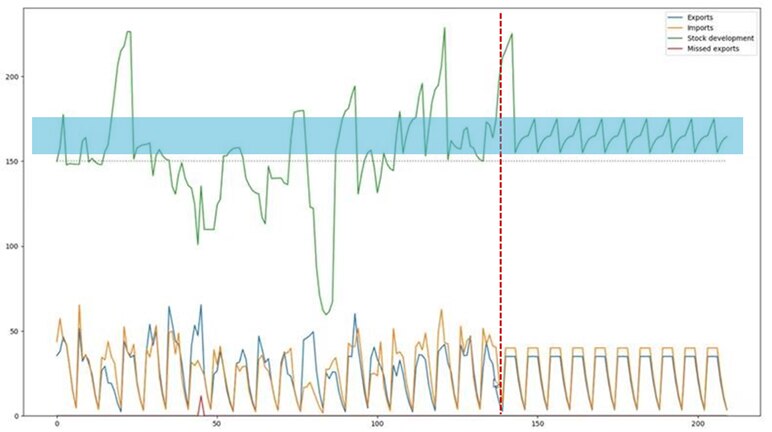
The below figures illustrate a simulation where stock is planned perfectly into the future, but how the volatility of the balance of trade can have a significant impact on the actual stock levels over time (see figure D). When adding a compliance range to evaluate how equipment was planned, the imbalance volatility has less significance when identifying how the target stock levels should be improved (see figure E).
|
|
Figure D: Future stock is planned perfectly and imbalance volatility impacts compliance negatively. | Figure E: Future stock is planned perfectly and imbalance volatility has a limited impact on compliance. |
Input Preparation
Setting the Standard Deviation
To calculate the above metrics, the standard deviation valuation must be transformed from the original forecast data into a meaningful value, useful for the site-level TSL calculations. Because we assume that site level forecast is dependent/correlated + it is more important that buffers are correct on pool level, we simply split the standard deviation from pool to site, using Split Ratios. To even out any noise in the site level standard deviations, a window function is applied to smooth out the values across the weeks. This is done by setting the standard deviation of week x as an average of x-1, x and x+1 (i.e. 3 weeks total).
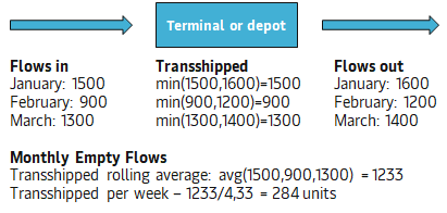
Transshipment Calculation
The transshipments are recalculated weekly using the below steps.
- Based on OTTs, all empty flow in and out are captured for each site, for the past three months.
Three months are used to capture - The transshipment are captured as the lowest value of flows in and flows out.
- The rolling monthly average is set as an average of the past three months
- The monthly target transformed to week by dividing the count with 4,33

Why a rolling average?
The transshipment figures for future target stock level could also be set based on planned OTTs. Due to feasibility of planning, it was agreed that a rolling average would be better fit for purpose. Furthermore, transshipments are purposefully captured per month and not per week to correctly capture cases where transshipment happens over more than one week (e.g. discharge in week 10 and load in week 11).
How are OTTs identified and used?
To identify transshipments within a week, OriginDeparture timestamp is used for units being loaded, and DestinationDeparture is used for units being discharged. As these timestamps are only available for marine, FromDate/ToDate will be used for Load/Discharge respectively, as a fallback to capture correct timestamps for inland OTTs.
OTTs in state Cancelled and OTTs that are not matched with GSIS are ignored.
Inputs and Formulas
Metrics
The TSL calculations uses a multiple inputs for the target stock level model. The main inputs used for the calculations are described below.
| Forecast type | Metric | Source | Alias | Formula |
|---|---|---|---|---|
| Export Pick-Up | Auto Prediction | Auto Forecast | aExpP | - |
| Standard Deviation | Auto Forecast | aExpStd | - | |
| Manual Prediction | User Input | mExp | - | |
| Effective Prediction | Calculated | eExpP | IF (mExpP <> NULL) THEN mExpP ELSE aExpP | |
| Import Return | Auto Prediction | Auto Forecast | aExpP | - |
| Standard Deviation | Auto Forecast | aImpStd | - | |
| Manual Prediction | User Input | mImpP | - | |
| Effective Prediction | Calculated | eImpP | IF (mImpP <> NULL) THEN mImpP ELSE aImpP | |
| Balance of Trade | Effective Prediction | Calculated | botp | eImpP - eExpP |
| Standard Deviation | Calculated | botstd | √(aExpStd² + aImpStd²) |
Input Parameters
The input parameters used in the TSL calculations, are described in below table. The parameters can be set and managed per site and equipment type. The input parameters are used to manage buffers individually.
| Input | Alias | Description | Used to Manage | Default Value |
|---|---|---|---|---|
| Equipment Preparation Days | epd | The number of days required to prepare each unit for import/export. | Equipment Preparation Buffer | 3 |
| Z value | z | The Z value is applied to the standard deviation to set the confidence interval. | Imbalance Volatility Buffer | 1,65 |
| Days Without Supply | dws | Accepted days without supply, used to manage the required buffer for deficit locations. | Supply Reliability Buffer | 7 |
| Balance of Trade Days | botd | Number of days of the weekly balance of trade to keep as buffer. | Balance of Trade Buffer | 7 |
Buffers
| Buffer | Description | Formulas | ||||||||||||||||
|---|---|---|---|---|---|---|---|---|---|---|---|---|---|---|---|---|---|---|
| Equipment Preparation | This buffer considers the stock level required to turn empty equipment and prepare it for next destination. It takes the max of imp/exp to recognize preparation requirements for any site. The result is transformed to a daily stock target, using the Equipment Preparation Days (epd) input parameter. | turns = max( eImpP; eExpP) weekspread = epd/7 equ_prep = turns * weekspread | ||||||||||||||||
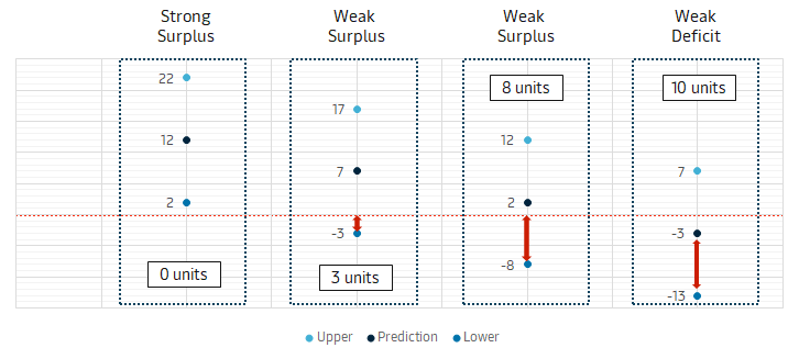
| Imbalance Volatility | This buffer considers the volatility in the balance of trade and keeps a buffer if the imbalance is negative (i.e. site has deficit behavior) and the buffer is not applied to sites with a strong surplus. The buffer required is set by adjusting the Z value (z) input parameter. To help understand the formulas, we can some typical imbalance behaviors and related buffer illustrated below:
List of z values with associated confidence intervals..
| deviation = botstd * z lower = botp - deviation imb_vol = IF (botp < 0) THEN deviation ELSE -min(lower; 0) | ||||||||||||||||
| Supply Reliability | This buffer considers the supply requirement (i.e. inbound OTTs) for deficit locations. The buffer keeps part of the weekly supply demand, based on the Days Without Supply (dws) parameter. | def_bot = max(-botP; 0) weekspread = dws/7 sup_rel = def_bot * weekspread | ||||||||||||||||
| Balance of Trade | This buffer sets the upper bound of the target stock level to consider the volatility of the stock level over time. The buffer keeps part of the weekly supply demand, based on the Balance of Trade Days (botd) parameter. | weekspread = botd/7 bot = abs(botp) * weekspread | ||||||||||||||||
| Transshipments | This buffer represents all the empty flows in and out of site stock, that are not used for the local demand. The transshipments are calculated automatically, but manual overrides are possible in the Manage TSL screen. The transshipments is recalculated once every week using OTT Load and Discharge numbers (see Reconciliation). It is possible to overwrite the automatically calculated value from the front-end. | - | ||||||||||||||||
| Smoothing | This buffer is added as part of the calculations by smoothing the TSL MAX target from week to week, giving a better transition over time, making planning more feasible and compliance more fair. The smoothing component is calculated in using a window function (in this case, in SQL). The smoothed max takes a 3-week rolling average from 1 preceding to 1 following week. The smoothing capped to never be lower than than the TSL max, prior to the smoothing. Similarly, the smoothing of the compliance max is also capped to never be lower than smoothed TSL max. | - |

Calculations
This section describes how the target stock levels are set using the defined buffers, and how the targets should be combined and aggregated across multiple sites and equipment types in order to analyse them correctly.
Setting TSL MIN and TSL MAX
The target stock levels are set on site/equipment type level by first calculating the buffers and adding them together. An additional step is added when setting the targets, which is adding a smoothing the TSL MAX value. The compliance targets are set using the standard deviation of the balance of trade (botstd), by adding one on top of the max and subtracting one from the min. The compliance max is also smoothed across weeks using a similar approach as the one smoothing the TSL MAX. The formulas to set the MIN and MAX are captured below.
| Formulas | tsl_min = equprep + imbvol + suprel ctsl_min = tsl_min - botstd |
Aggregation of Targets
Stock is generally planned to be within the bounds of the target stock levels (i.e. min and max). On average, this means that the target stock level will be around the middle of the bounds and hit the bounds only occasionally. Consequently, it is expected that the aggregated stock will center around the middle of the aggregated target stock levels. Because we can understand the target stock level range as having a mean and a normally distributed spread, we can also combine the targets using the Pythagorean Theorem of Statistics, which specifies that for independent variables, their individual variances can be added together.
This approach requires us to capture the variances for each target stock level we want to include in our aggregation. Furthermore, due to the smoothing function of the max targets it is necessary to capture the variances between the mean to the upper and lower bound (i.e. min and max) separately. The variance is set as the squared deviation, representing the distance from the mean to the relevant bound.
| Component | Alias | Formula |
|---|---|---|
| Middle Point | tsl_mid | tsl_mid = (tsl_min + tsl_max)/2 |
| TSL Min Variance | tsl_min_var | tsl_min_var = (tsl_mid - tsl_min)² |
| TSL Max Variance | tsl_max_var | tsl_max_var = (tsl_max - tsl_mid)² |
| Compliance Min Variance | ctsl_min_var | ctsl_min_var = (tsl_mid - ctsl_min)² |
| Compliance Max Variance | ctsl_max_var | ctsl_max_var = (ctsl_max - tsl_mid)² |
The combined targets are set by first capturing the combined deviation as the square root of the combined variances and then subtracting the value from the combined middle point.
| Component | Alias | Formula |
|---|---|---|
| Combined Middle Point | tsl_cmid | tsl_cmid = ⅀ tsl_mid, across targets |
| Combined TSL Min | tsl_cmin | tsl_cmin = tsl_cmid - √( ⅀ tsl_min_var, across targets) |
| Combined TSL Max | tsl_cmax | tsl_cmax = tsl_cmid - √(⅀ tsl_max_var, across targets) |
| Combined Compliance Min | ctsl_cmin | ctsl_cmin = tsl_cmid - √(⅀ ctsl_min_var, across targets) |
| Combined Compliance Max | ctsl_cmax | ctsl_cmax= tsl_cmid - √(⅀ ctsl_max_var, across targets) |